Inset maps with insetplot

This vignette shows how to compose ggplot2 maps with insets using insetplot, with emphasis on runnable code.

Quick start

# 1) Configure the layout: one main map + one inset (nc loaded in setup)
config_insetmap(
    data_list = list(nc),
    specs = list(
        inset_spec(main = TRUE),
        inset_spec(
            xmin = -82, xmax = -80.5, ymin = 35.5, ymax = 36, # bbox for the inset area
            loc = "left bottom", # where to place the inset
            scale_factor = 2 # size relative to main
        )
    )
)

# 2) Build a base plot (shared by main and inset unless a spec supplies its own)
base <- ggplot(nc, aes(fill = AREA)) +
    geom_sf() +
    scale_fill_viridis_c() +
    guides(fill = "none") +
    theme_void()

# 3) Compose
with_inset(base)

# 4) Save with correct aspect ratio (only width or height is needed)
# ggsave_inset("inset_map.png", width = 10)

You can also provide custom plots per spec, then call with_inset() without a plot argument.

For example, you may want to add some annotations to the inset(s) only.

main <- ggplot(nc, aes(fill = AREA)) +
    geom_sf() +
    scale_fill_viridis_c() +
    guides(fill = "none") +
    theme_void()

config_insetmap(
    data_list = list(nc),
    specs = list(
        inset_spec(main = TRUE, plot = main),
        inset_spec(
            xmin = -82, xmax = -80.5, ymin = 35.5, ymax = 36,
            loc = "left bottom", # where to place the inset
            scale_factor = 2, # size relative to main
            plot = main +
                annotate("label", x = -80.5, y = 35.5, label = "Detail", size = 5, hjust = 1, vjust = 0, fill = "white", size.unit = "pt")
        )
    )
)
with_inset()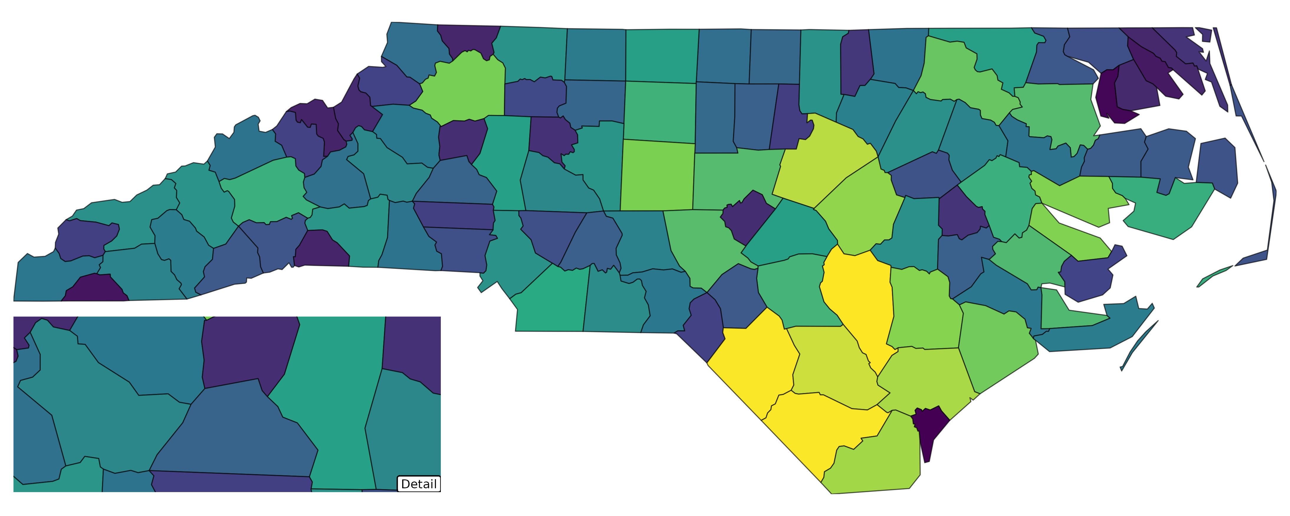

Why insetplot (vs. using cowplot/patchwork directly)

But why not just use patchwork::inset_element() or cowplot::draw_plot() directly? I’ll demonstrate this by the following minimal example.

First, without insetplot, we should manually create the inset plot by zooming into the desired bbox like this (I add borders to plots for clarity):

inset_bbox <- c(xmin = -82, xmax = -80.5, ymin = 35.5, ymax = 36)
main_map <- ggplot(nc, aes(fill = AREA)) +
    geom_sf() +
    scale_fill_viridis_c() +
    guides(fill = "none") +
    theme_void() +
    map_border(linewidth = 0.5)
inset_map <- main_map +
    coord_sf(
        xlim = c(inset_bbox["xmin"], inset_bbox["xmax"]),
        ylim = c(inset_bbox["ymin"], inset_bbox["ymax"])
    )

Suppose we want to add the inset at the bottom-left corner with height 30% of the main plot.

Now, let’s try patchwork::inset_element(). Since, here, we don’t know the correct aspect ratio, we might specify arbitrary width/height for the inset.

# Manual insetting with patchwork: force a mismatched container ratio
main_map + patchwork::inset_element(
    inset_map,
    left = 0, bottom = 0, right = 0.3, top = 0.3, # arbitrary width/height
    align_to = "panel"
)

Inset via patchwork

And now cowplot::draw_plot():

cowplot::ggdraw(main_map) +
    cowplot::draw_plot(inset_map, 0, 0, 0.3, 0.3) # arbitrary width/height

Inset via cowplot

Thing will become much worse when you save the plots with different output apsect ratios. For example, if I save the above plot with a height-to-width artio of 1.0:

cowplot::ggdraw(main_map) +
    cowplot::draw_plot(inset_map, 0, 0, 0.3, 0.3) # arbitrary width/height

Inset via cowplot with wrong aspect ratio

You may get better results by adjusting the inset size manually based on visual inspection of the output plot.

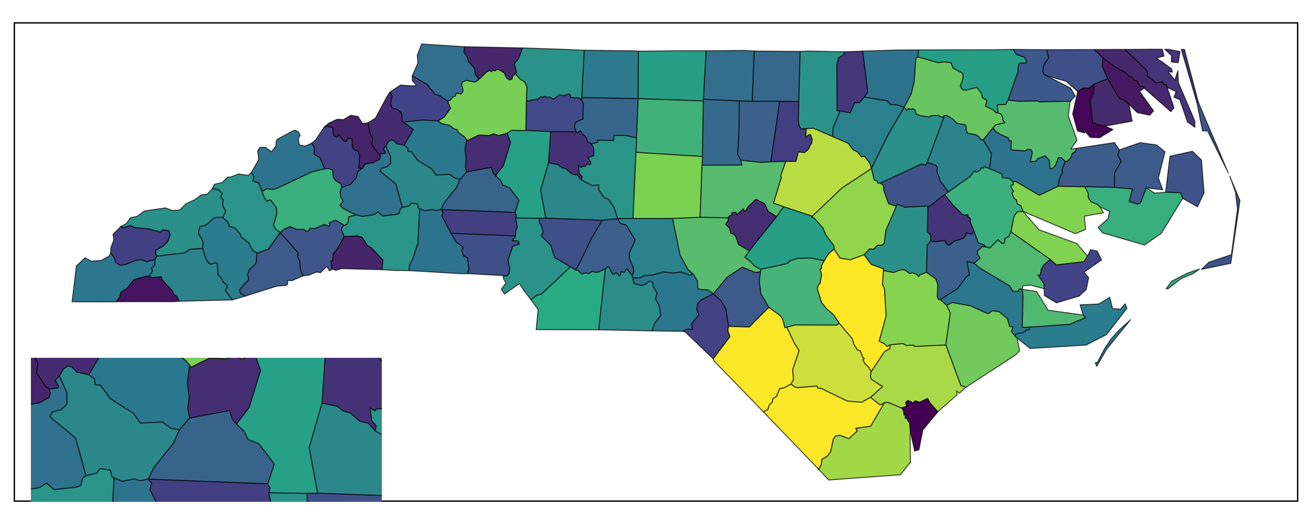
Now let’s see how insetplot handles this more gracefully.

config_insetmap(
    data_list = list(nc),
    specs = list(
        inset_spec(main = TRUE),
        inset_spec(
            xmin = -82, xmax = -80.5, ymin = 35.5, ymax = 36,
            loc = "left bottom", height = 0.3
        )
    )
)

# You even don't need to prepare `inset_map` here since insetplot handles it internally
with_inset(main_map)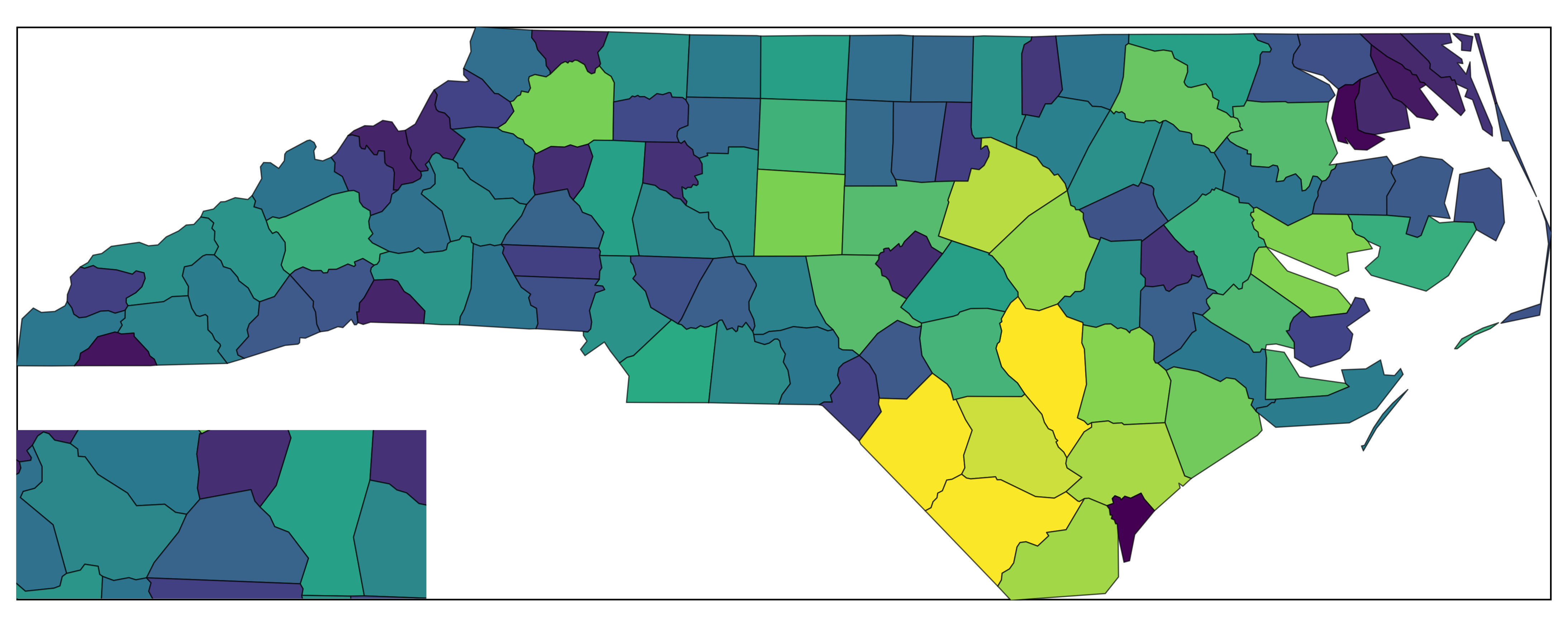

Inset via insetplot

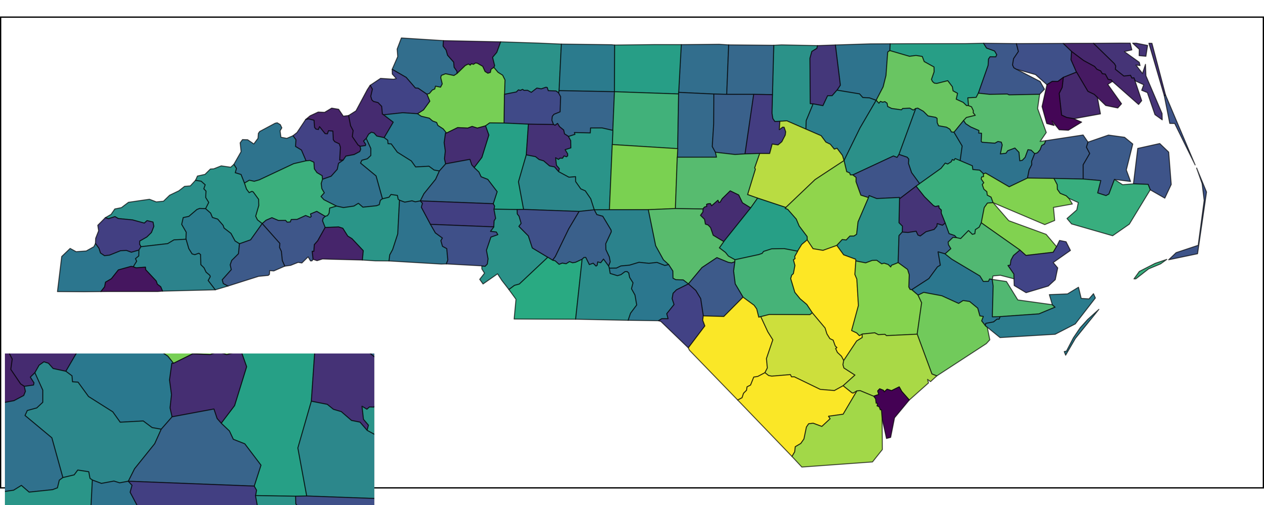
Even you save this plot with a not-that-good aspect ratio, such as 1.0:

with_inset(main_map)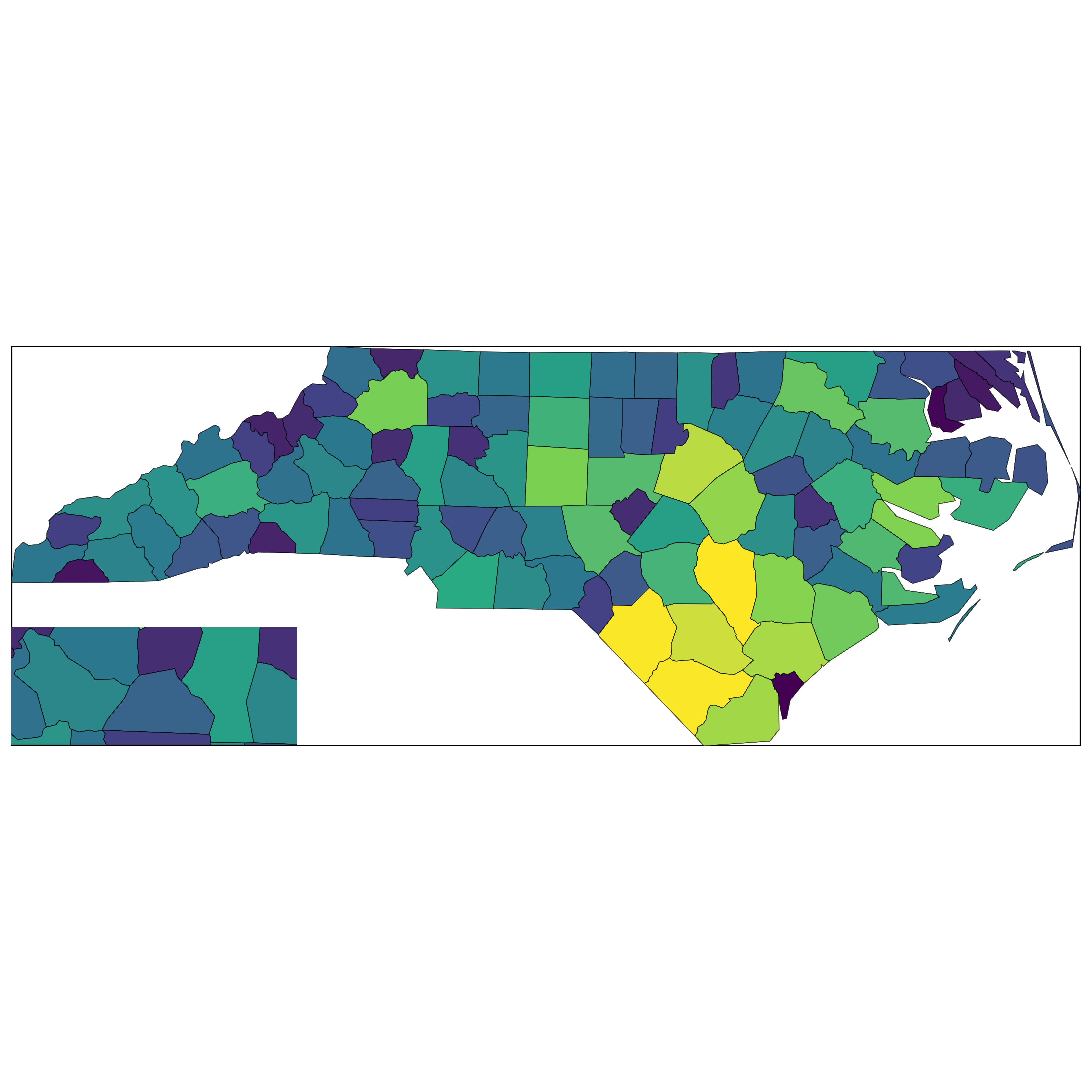

Inset via insetplot with wrong aspect ratio

And don’t forget that, in fact, you can always save it correctly with ggsave_inset().

In short: insetplot calculates inset sizes from data aspect ratios (via bounding boxes) and guides saving via ggsave_inset(), so you avoid accidental stretching.

What each parameter means

Below are the key functions and their arguments, illustrated inline.

Define subplots (inset_spec)

# Define a main spec (no size/position needed)
inset_spec(main = TRUE)

# Define an inset by bbox + position + size
inset_spec(
    xmin = -120, xmax = -100, ymin = 30, ymax = 50, # spatial extent (data CRS)
    loc = "right bottom", # shorthand position on full canvas
    width = 0.30 # size in [0,1]; prefer ONE of width/height
)

# Prefer scale_factor to size relative to main plot automatically
inset_spec(
    xmin = -120, xmax = -100, ymin = 30, ymax = 50,
    loc = "left bottom",
    scale_factor = 0.5 # relative to main ranges
)

inset_spec() arguments:

• xmin, xmax, ymin, ymax: numeric bbox of the subplot in data coordinates. Any NA is filled from overall extent.
• loc: convenience string “left|center|right bottom|center|top”. Ignored if loc_left/loc_bottom given.
• loc_left, loc_bottom: numbers in [0,1] for precise bottom-left position on the canvas.
• width, height: numbers in (0,1]. Recommend providing only one; the other is inferred to preserve spatial aspect.
• scale_factor: number in (0,Inf) to size inset relative to main plot’s x/y ranges. Overrides width/height when set.
• main: TRUE if this spec is the main plot (exactly one spec must be main).
• plot: optional ggplot for this spec; otherwise the shared base plot is used.

Configure layout (config_insetmap)

cfg <- config_insetmap(
    data_list = list(nc), # list of sf objects used to compute extents/CRS
    specs = list(
        inset_spec(main = TRUE),
        inset_spec(xmin = -84, xmax = -75, ymin = 33, ymax = 37, loc = "left bottom", scale_factor = 0.5)
    ),
    crs = sf::st_crs("EPSG:4326"), # target CRS for coord_sf()
    border_args = list(color = "black", linewidth = 1) # passed to map_border()
)

config_insetmap() arguments:

• data_list: list of sf objects; used to compute union bbox and main aspect ratio.
• specs: list of inset_spec objects; exactly one must have main = TRUE.
• crs: target CRS passed to ggplot2::coord_sf().
• border_args: style for inset borders via map_border().

Compose the figure (with_inset)

out <- with_inset(base) # returns the composed plot
names(with_inset(base, .return_details = TRUE)) # list with full, subplots, layouts, main_ratio
#> [1] "full"            "subplots"        "subplot_layouts" "main_ratio"

# You can also provide custom plots after configuring
out <- with_inset(list(main_map, inset_map))
#> Coordinate system already present.
#> ℹ Adding new coordinate system, which will replace the existing one.

with_inset() arguments:

• plot: a single ggplot used for all specs, or a list of ggplots per spec, or NULL if every spec has its own plot.
• .cfg: the configuration to use (defaults to last_insetcfg()).
• .as_is: return the input plot unchanged (handy for debugging/reuse).
• .return_details: return internals (layouts, subplots) instead of just the composed ggplot.

Save with the right ratio (ggsave_inset)

# Provide only width (or only height). The other dimension is computed to match the main ratio.
# ggsave_inset("map.png", p, width = 10)

ggsave_inset() arguments:

• width/height: only one is needed; the other is calculated from the configuration’s main ratio. If both are given, output may not match the intended ratio.
• ratio_scale: optional multiplier if extra space is needed for legends/titles.